1
The University of Oklahoma catalogue describes AME 2213 this way: “First and second law of thermodynamics are developed and applied to the solutions of problems from a variety of engineering fields. Extensive use is made of differential calculus to interrelate thermodynamics functions”. My interpretation of this description is more specific. Thermodynamics, generally speaking, is the science of energy. The transformation of energy from one form to another, and in many cases thermodynamics is about transforming heat into work, such as in an automobile engine or at a power plant.
The application of Thermodynamics is almost everywhere in our daily life. Examples of some application areas of this subject are: Propulsion, Internal Combustion Engines, Power Plants, Refrigeration and Air Conditioning, Solar Heating, Interaction of Human Body with Surroundings, Biomedical devices, Human body, animal, plants, Ecological systems, etc. In this course on thermodynamics we will focus on the analysis of energy systems and the application of these systems to real world contexts.
There are two approaches of teaching Thermodynamics – microscopic and macroscopic. Classical Thermodynamics (macroscopic approach) does not require detailed knowledge of molecular motion to describe a System. We will mainly use this approach in AME 2213. Statistical Thermodynamics (macroscopic approach) considers quantum mechanical description of molecules. We will occasionally use this approach to improve our basic understanding.
To understand the fundamental concepts of thermodynamics, basic principles (conservation of mass, conservation of energy, concept of entropy) and basic thermodynamics terminology (System, Property, State, Equilibrium, Process, Pressure) should be learn. This first chapter is dedicated to these introductory concepts, as well as to the importance of dimensions and units. We will distinguish primary dimensions in Thermodynamics such as mass (m), length (L), time (t), temperature (T), electric current (I), luminous intensity (lv), amount of substance (n), and secondary dimensions (derived) such as: velocity ( ), volume (
 ), etc. In this course we will use two important unit systems: English (E) and International System of Units (SI).
Thermodynamics and Energy
Thermodynamics is the science of energy, including energy storage and energy in transit. The Conservation of Energy Principle states that energy cannot be created or destroyed, but can only change its form. The three forms of energy storage of greatest interest to us are Potential Energy (PE), Kinetic Energy (KE), and Internal Energy (U), which we introduce below. The two forms of energy in transit that we consider are Work (W) and Heat (Q), and the interactions between these various forms of energy are defined in terms of the First Law of Thermodynamics.
Force and Work
Newton’s Second Law states:
![\[F[N]=ma\left[kg\times\frac{m}{s^2}\right]\]](https://pressbooks.pub/app/uploads/quicklatex/quicklatex.com-e6d01ad21359c0d668928f9756dee59a_l3.png "Rendered by QuickLaTeX.com")
where: F is the force in Newtons [N]
m is the mass in kilograms [kg]
a is the acceleration in meters per second squared ![\left[\frac{m}{s^2}\right]](https://pressbooks.pub/app/uploads/quicklatex/quicklatex.com-5d56c6f44e04298306faf136191e7534_l3.png "Rendered by QuickLaTeX.com")
Here we define a pound mass (lbm) and a pound force (lbf), thus since the acceleration due to gravity g = 32.2![\left[\frac{ft}{s^2}\right]](https://pressbooks.pub/app/uploads/quicklatex/quicklatex.com-abbc5f8b5a8f9af88b6d592173db2c1b_l3.png "Rendered by QuickLaTeX.com") we have:
we have:
![\[1\:lbf\:=\left[\frac{32.2\:lbm\:ft}{s^2}\right]\]](https://pressbooks.pub/app/uploads/quicklatex/quicklatex.com-db8850fd491acb6a18bb6186db3ed3e9_l3.png "Rendered by QuickLaTeX.com")
![\[1\:slug\:=32.2\:lbm\]](https://pressbooks.pub/app/uploads/quicklatex/quicklatex.com-1042d6742b0a0a3d84b77ad7584df39e_l3.png "Rendered by QuickLaTeX.com")
Unity Conservation Ratio:
![\[\frac{N\times s^2}{kg\times m}=1\,\,\,\,\,\text{and}\,\,\,\,\,\frac{lbf\times s^2}{32.174,lbm\times ft}=1\]](https://pressbooks.pub/app/uploads/quicklatex/quicklatex.com-d3004c95be753850a4fe7f1d33bdde82_l3.png "Rendered by QuickLaTeX.com")
We now consider the work done (W), the energy in transit requiring both the applied force (F) and movement (x). If the force (F) is constant over the distance moved (x) then the work done is given by:
![\[W[J]=F\times x[Nm]\]](https://pressbooks.pub/app/uploads/quicklatex/quicklatex.com-a571be89cc0269a0cbd660f90124c92d_l3.png "Rendered by QuickLaTeX.com")
where: W is the work done in Joules [J]
F is the force in Newtons [N]
x is the distance moved in meters [m]
However, in general the force (F) is not constant over the distance x, thus we need to sum all the incremental work processes taking into consideration the variation of the force (F). This leads to the equivalent integral form for determining work done (W) as follows:
![\[W[J]=\int F\,dx\]](https://pressbooks.pub/app/uploads/quicklatex/quicklatex.com-8813be3bb402c93ff31c7fbf70152a1d_l3.png "Rendered by QuickLaTeX.com")
where: W is the work done in Joules [J]
F is the force in Newtons [N]
x is the distance moved in meters [m]
SI and English Units

![g \approx 9.81\left[\frac{\si\m}{\si\s^2}\right]\approx 32.2\left[\frac{\si{ft}}{\si\s^2}\right] \implies 1\left[\si\m \right]=3.28 \left[\si{ft}\right]](https://pressbooks.pub/app/uploads/quicklatex/quicklatex.com-1d3e564dbe932d53c3b4354c782fe713_l3.png "Rendered by QuickLaTeX.com")
![4 \left[\frac{\si\m}{\si\s}\right] \approx 9\left[\frac{\si{miles}}{\si{hour}}\right] \iff 80 \left[\frac{\si\km}{\si{hour}}\right] \approx 50\left[\frac{\si{miles}}{\si{hour}}\right]](https://pressbooks.pub/app/uploads/quicklatex/quicklatex.com-cff3349bc25c159db54fb2fb6c8799a8_l3.png "Rendered by QuickLaTeX.com")
Mass, Volume
![1[\si\kg] \approx 2.2[\si{lbm}]](https://pressbooks.pub/app/uploads/quicklatex/quicklatex.com-71ad209fae208706390aa66acfe0992b_l3.png "Rendered by QuickLaTeX.com")
![1[\si\m^3] \text{ water} \approx 1000[\si\kg] \implies 1 \text{ Liter water} \approx 1[\si\kg]](https://pressbooks.pub/app/uploads/quicklatex/quicklatex.com-64e9a80906a2d34525878718871d9b59_l3.png "Rendered by QuickLaTeX.com")
![1[\si\m^3] \text{ air} \approx 1.2[\si\kg]](https://pressbooks.pub/app/uploads/quicklatex/quicklatex.com-b0ce807c4ba3223026f189801a9b949e_l3.png "Rendered by QuickLaTeX.com")
![1 \ [\si{kJ}] \ (\si{kiloJoule}) \approx 1 [\si{BTU}] \ (\text{British Thermal Unit})](https://pressbooks.pub/app/uploads/quicklatex/quicklatex.com-8d749aa0fbac0aeba56a36632e209a55_l3.png "Rendered by QuickLaTeX.com")
![\nicefrac{3}{4} \ [\si{kW}] \ (\si{kiloWatt}) \approx 1 [\si{hp}] (\text{Horse Power})](https://pressbooks.pub/app/uploads/quicklatex/quicklatex.com-26100aca1467d2838c08341ee436432a_l3.png "Rendered by QuickLaTeX.com")
more correctly:
![1 \ [\si{kJ}] = 1.055 \ [\si{BTU}]](https://pressbooks.pub/app/uploads/quicklatex/quicklatex.com-a85128462a671131fb0cce120a5cb2b6_l3.png "Rendered by QuickLaTeX.com")
![0.746 \ [\si{kW}] = 1 \ [\si{hp}]](https://pressbooks.pub/app/uploads/quicklatex/quicklatex.com-d00b3ac6f4df865e41dc0b55ece80125_l3.png "Rendered by QuickLaTeX.com")
![\text{Weight of one small apple}\approx 1 [\si\N] (\text{Newton})](https://pressbooks.pub/app/uploads/quicklatex/quicklatex.com-04496597b91bab7757dff485ca312d4c_l3.png "Rendered by QuickLaTeX.com")
![\text{Area of a SI standard card table}\approx 1[\si\m^2]](https://pressbooks.pub/app/uploads/quicklatex/quicklatex.com-c7418deefeaa0669a0b8cbeffa31e342_l3.png "Rendered by QuickLaTeX.com")
![\text{Pressure due to apple sauce made from a single apple spread evenly across the card table}\approx 1 \ [\si{Pa}] \ (\text{Pascal})](https://pressbooks.pub/app/uploads/quicklatex/quicklatex.com-31c0ea21a276e7123dbedd52d5774ac4_l3.png "Rendered by QuickLaTeX.com")
![1[\si{bar}]=100[\si{kPa}]\approx 14.5 \left[\frac{\si{lbf}}{\si{in}^2}\right] (\si{psi})](https://pressbooks.pub/app/uploads/quicklatex/quicklatex.com-dc8d4576b80d78096b79590354e9f472_l3.png "Rendered by QuickLaTeX.com")
Quick Quiz
We all know (from reading our speedometers) that 50 mph is equivalent to 80  .
.
- What is the accuracy of this conversion?
- Use this information to show that 9 mph is equivalent to 4 .
We find that with the above survival kit we can determine many unit conversions between SI & English units, typically as demonstrated in the following block:


![1 \ \si\m^3 \left[ \left( \frac{32.2 \ \si{ft}}{9.81 \ \si\m} \right)^3 \right]=35.36 \ \si{ft}^3](https://pressbooks.pub/app/uploads/quicklatex/quicklatex.com-ec79cfda64341d24344ccc96c220f8f7_l3.png "Rendered by QuickLaTeX.com")
![1 \ \si{lbf} \left[ \nicefrac{ \frac{32.2 \ \si{lbm \ ft}}{\si\s^2}}{\si{lbf}}\right] \left[\frac{\si\kg}{2.2 \ \si{lbm}}\right] \left[\frac{9.81 \text{ m}}{32.2 \text{ ft}} \right] \left[ \nicefrac{\text{N}}{\frac{\text{kg m}}{\text{s}^2}}\right]=4.46 \text{ N}](https://pressbooks.pub/app/uploads/quicklatex/quicklatex.com-bd1deda67eddde2b1463826c268a8fe6_l3.png "Rendered by QuickLaTeX.com")
Forms of Energy
The various forms of energy of interest to us are introduced in terms of a solid body having a mass m [kg]. These include potential, kinetic and internal energy. Potential energy (PE) is associated with the elevation of the body, and can be evaluated in terms of the work done to lift the body from one datum level to another under a constant acceleration due to gravity g, as follows:
![\[W=\int_{h_1}^{h_2}F\,dx=\int_{h_1}^{h_2}m\times g\,dx=m\times g(h_2-h_1)=m\times\Delta pe=\Delta PE\]](https://pressbooks.pub/app/uploads/quicklatex/quicklatex.com-e4ed405f7f0ec3d01f8b76f590b09f6d_l3.png "Rendered by QuickLaTeX.com")
Kinetic energy (KE) of a body is associated with its velocity ![\vec{V}\left[\frac{m}{s}\right]](https://pressbooks.pub/app/uploads/quicklatex/quicklatex.com-63cb9b0cc28c0105d21b95a294368e2f_l3.png "Rendered by QuickLaTeX.com") and can be evaluated in terms of the work required to change the velocity of the body, as follows:
and can be evaluated in terms of the work required to change the velocity of the body, as follows:
![\[W=\int F\,dx=\int m\times a \,dx=\int m\times\frac{d\vec{V}}{dt}dx\]](https://pressbooks.pub/app/uploads/quicklatex/quicklatex.com-006b90fc3871b63f775b48cd2a87cff9_l3.png "Rendered by QuickLaTeX.com")
however, velocity  , thus integrating from
  :
:
![\[W=\int_{\vec{V_1}}^{\vec{V_2}}m\times\vec{V}\,d\vec{V}=m\times\left(\frac{\vec{V}_2^2-\vec{V}_1^2}{2}\right)=m\times\Delta ke=\Delta KE\]](https://pressbooks.pub/app/uploads/quicklatex/quicklatex.com-4578de09dc32fec7970010cb72f7ec5a_l3.png "Rendered by QuickLaTeX.com")
Internal energy (U) of a body is that associated with the molecular activity of the body as indicated by its temperature T [°C], and can be evaluated in terms of the heat required to change the temperature of the body having a specific heat capacity C![\left[\frac{J}{kg\times°C}\right]](https://pressbooks.pub/app/uploads/quicklatex/quicklatex.com-7ce0477be09f747abe39223c744bfdee_l3.png "Rendered by QuickLaTeX.com") , as follows:
, as follows:
![\[Q=m\times C\times\Delta T=m\times\Delta u=\Delta U\]](https://pressbooks.pub/app/uploads/quicklatex/quicklatex.com-e433f345a7a7dd52b4837de8e255a743_l3.png "Rendered by QuickLaTeX.com")
Cooking with Potential Energy
In order to gain an intuitive appreciation for the relative magnitudes of the different forms of energy we consider the (tongue-in-cheek) example of an attempt to cook a turkey by potential energy. The turkey is brought to the top of a 100 m building (about 30 stories) and then dropped from the ledge. The potential energy is thus converted into kinetic energy, and finally on impact the kinetic energy is converted into internal energy. The increase in internal energy is represented by an increase in temperature, and hopefully, if this experiment is repeated enough times the temperature increase will allow the turkey to cook. This remarkable experiment was first reported by R.C.Gimmi and Gloria J Browne – “Cooking with Potential Energy“, published in the Journal of Irreproducible Results (Vol. 33, 1987, pp 21-22).

Potential Energy


Internal Energy


![\[\color{red}\boxed{\color{black}W=\frac{m \cdot \vec{V}^2}{2}=\Delta KE}\]](https://pressbooks.pub/app/uploads/quicklatex/quicklatex.com-ee091f6edcf365e2905451ced04146ca_l3.png "Rendered by QuickLaTeX.com")
Equating all three energy forms:
![\Delta PE = \Delta KE = \Delta U \ [\si\J]](https://pressbooks.pub/app/uploads/quicklatex/quicklatex.com-fed2c6bfdaa09fcfff4cd9ff348e2934_l3.png "Rendered by QuickLaTeX.com")

Since mass m is common, evaluate specific energy (h=100 m):
![\Delta pe = \Delta ke = \Delta u \ [\si{\J / \kg}]](https://pressbooks.pub/app/uploads/quicklatex/quicklatex.com-3258431490ceaead1e898e7d5ee6de59_l3.png "Rendered by QuickLaTeX.com")
![g \cdot h = \frac{\vec{V}^2}{2} = C \cdot \Delta T \approx 1000 \ [\si{\J / \kg}]](https://pressbooks.pub/app/uploads/quicklatex/quicklatex.com-547a4ce930297768863cf1768b4b73c7_l3.png "Rendered by QuickLaTeX.com")
![\frac{\vec{V}^2}{2} \left[\frac{\si\m^2}{\si\s^2}\right] = 1000 \left[ \frac{\si\J}{\si\kg} \cdot \frac{\si{\N\m}}{\si\J} \cdot \frac{\si{\kg\m}}{\si{\s}^2} \cdot \frac{1}{\si\N}\right]](https://pressbooks.pub/app/uploads/quicklatex/quicklatex.com-dca112a07a6eb823789c4d14702f3320_l3.png "Rendered by QuickLaTeX.com")
![\vec{V}_{\text{impact}} = \sqrt{2000} = 44.7 \left[ \nicefrac{\si\m}{\si\s}\right] (\approx 100 \ \si{mph}!)](https://pressbooks.pub/app/uploads/quicklatex/quicklatex.com-5e8f4587b20ed669d1fea48f2cb2bc48_l3.png "Rendered by QuickLaTeX.com")
We estimate the specific heat of a turkey.
![C = 3000 \ [\si{\J / \kg \ ^{\circ}C}]](https://pressbooks.pub/app/uploads/quicklatex/quicklatex.com-fa65a07b8d582c944325f50867b4a762_l3.png "Rendered by QuickLaTeX.com")
Thus
![C \Delta T = 3000 \ \Delta T = 1000 \ [\si{\J / \kg}] \implies \color{red}\boxed{\color{black} \Delta T = 0.33 ^{\circ}C}](https://pressbooks.pub/app/uploads/quicklatex/quicklatex.com-395da7c5707d54f6203208c643b0e1d2_l3.png "Rendered by QuickLaTeX.com")
What a disappointment! At 0.33°C per fall it will require repeating the experiment 600 times just to reach the cooking temperature of 200°C.
Thermodynamics Systems
For purposes of analysis we consider two types of Thermodynamic Systems:
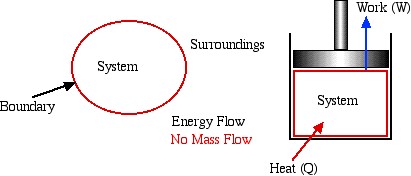
- Closed System – usually referred to as a System or a Control Mass. This type of system is separated from its surroundings by a physical boundary. Energy in transit in the form of Work or Heat can flow across the system boundary, however there can be no mass flow across the boundary. One typical example of a system is a piston / cylinder device in which the system is defined as the fixed mass of fluid contained within the cylinder.
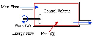
- Open System – usually referred to as a Control Volume. In this case, in addition to work or heat, we have mass flow of the working fluid across the system boundaries through inlet and outlet ports. In this course we will be exclusively concerned with steady flow control volumes, in that the net mass of working fluid within the system boundaries remains constant (i.e. mass flow in
![\left[\frac{kg}{s}\right]](https://pressbooks.pub/app/uploads/quicklatex/quicklatex.com-47a834cfbc06b948e06feac5e5d40c8b_l3.png "Rendered by QuickLaTeX.com") = mass flow out ). The following sections refer mainly to systems – we will consider control volumes in more detail starting with Chapter 4.
= mass flow out ). The following sections refer mainly to systems – we will consider control volumes in more detail starting with Chapter 4.


Properties of a System
The closed system shown above can be defined by its various Properties, such as its pressure (P), temperature (T), volume (V) and mass (m). We will introduce and define the various properties of thermodynamic interest as needed in context. Furthermore the properties can be either Extensive or Intensive (or Specific). An extensive property is one whose value depends on the mass of the system, as opposed to an intensive property (such as pressure or temperature) which is independent of the system mass. A specific property is an intensive property which has been obtained by dividing the extensive property by the mass of the system. Two examples follow – notice that specific properties will always have kilograms (kg) in the units’ denominator.
Specific volume:![\,v\left[\frac{m^3}{kg}\right]=\frac{volume\,V[m^3]}{mass\,m[kg]}](https://pressbooks.pub/app/uploads/quicklatex/quicklatex.com-ba45b1ac673d38777e9dd4edf0c59a3b_l3.png "Rendered by QuickLaTeX.com")
Specific internal energy:![\,u\left[\frac{kJ}{kg}\right]=\frac{internal\,energy\,U[m^3]}{mass\,m[kg]}](https://pressbooks.pub/app/uploads/quicklatex/quicklatex.com-f8bd0a1334fe2e1f01d060bd0b64d553_l3.png "Rendered by QuickLaTeX.com")
State and Equilibrium
The State of a system is defined by the values of the various intensive properties of the system.
The State Postulate states that if two independent intensive property values are defined, then all the other intensive property values (and thus the state of the system) are also defined. This can significantly simplify the graphical representation of a system, since only two-dimensional plots are required. Note that pressure and temperature are not necessarily independent properties, thus a boiling liquid will change its state from liquid to vapor at a constant temperature and pressure.
We assume that throughout the system Equilibrium conditions prevail, thus there are no temperature or pressure gradients or transient effects. At any instant the entire system is under chemical and phase equilibrium.
Process and Cycle
A Process is a change of state of a system from an initial to a final state due to an energy interaction (work or heat) with its surroundings. For example in the following diagram the system has undergone a compression process in the piston-cylinder device.

The Process Path defines the type of process undergone. Typical process paths are:
- Isothermal (constant temperature process)
- Isochoric or Isometric (constant volume process)
- Isobaric (constant pressure process)
- Adiabatic (no heat flow to or from the system during the process)
We assume that all processes are Quasi-Static in that equilibrium is attained after each incremental step of the process.
A system undergoes a Cycle when it goes through a sequence of processes that leads the system back to its original state.
Pressure
The basic unit of pressure is the Pascal [Pa], however practical units are kilopascal [kPa], bar [100 kPa] or atm (atmosphere) [101.32 kPa]. The Gage (or Vacuum) pressure is related to the Absolute pressure as shown in the diagram below:

1 Pascal ![\left[\si{\Pa}\right] = 1 \left[\frac{\si\N}{\si\m^2}\right]](https://pressbooks.pub/app/uploads/quicklatex/quicklatex.com-d3ea33514610ef97c2a25356af36a7b0_l3.png "Rendered by QuickLaTeX.com")
1 ![\left[\si{\bar}\right] = 10^5\left[\si{\Pa}\right]=100\left[\si{\kPa}\right]](https://pressbooks.pub/app/uploads/quicklatex/quicklatex.com-8a4f70f255d06f116c16a7d1914d0a19_l3.png "Rendered by QuickLaTeX.com")
1 ![\left[\si{atm}\right] = 101.32\left[\si{\kPa}\right]](https://pressbooks.pub/app/uploads/quicklatex/quicklatex.com-0d9e8d217d57b2511c0abe581136dd64_l3.png "Rendered by QuickLaTeX.com")
The basic method of measuring pressure is by means of a Manometer, as shown below:


 density of the liquid
 ![\left[ \nicefrac{\si\kg}{\si\m^3}\right]](https://pressbooks.pub/app/uploads/quicklatex/quicklatex.com-fe7e797660f8c7e5f8dab66a8467985b_l3.png "Rendered by QuickLaTeX.com")
 volume
 ![\left[\si\m^3\right]](https://pressbooks.pub/app/uploads/quicklatex/quicklatex.com-13e844cc9293850439d22e50aec6f7b6_l3.png "Rendered by QuickLaTeX.com")
 gravity acceleration
 ![\left[ 9.81\nicefrac{\si\m}{\si\s^2}\right]](https://pressbooks.pub/app/uploads/quicklatex/quicklatex.com-6269d62d45f23326ba52788e36bdf651_l3.png "Rendered by QuickLaTeX.com")
From a force balance:

Thus:


The atmospheric pressure is measured by means of a Mercury Barometer as follows:

Density of Mercury:
![\color{red}\boxed{\color{black}\rho_{\text{Hg}} \approx 13,600\left[\frac{\si\kg}{\si\m^3}\right]}](https://pressbooks.pub/app/uploads/quicklatex/quicklatex.com-605d35bf384204b02b4ef7b262f692d6_l3.png "Rendered by QuickLaTeX.com")
![\rho_{Hg} = (13595-2.47 \si{T} \left[^{\circ}\si{C}\right]) \left[\frac{\si\kg}{\si\m^3}\right]](https://pressbooks.pub/app/uploads/quicklatex/quicklatex.com-69ba924477b958d62f6820be0e5fcf8a_l3.png "Rendered by QuickLaTeX.com") (empirical)
(empirical)

Standard Atmosphere is defined as:

![P_{\text{atm}}=101.32 \left[\si{\kPa}\right]](https://pressbooks.pub/app/uploads/quicklatex/quicklatex.com-9a1732049b831832cf1065143b3518ed_l3.png "Rendered by QuickLaTeX.com")
Solved Problem 1.1 – Using a Barometer to determine the Height of a Building.
In this problem we use the basic mercury barometer to determine the height of a building. Consider the case that the barometer reading at the top of the building is 751 mm Hg, and at the bottom of the building is 760 mm Hg. Assume the density of mercury  , and that the average density of the column of air
  .
.
The approach to solution is illustrated in the following diagram. A free-body force diagram on the column of air allows us to determine the height as a function of the pressure difference ΔP from top to bottom.


Well, exactly 100m? – obviously this is a contrived example. When we first evaluated the height we came up with the result:
![]()
![\[ \text{height}=\color{red}\cancelto{\text{Nonsense!}}{\text{\color{black}100.209057}} \color{black}\ \si\m \ (\pm 1 \ \mu \si\m \ \text{?}) \]](https://pressbooks.pub/app/uploads/quicklatex/quicklatex.com-c2e3b86434dd23bc31ce0ff46ba791d9_l3.png "Rendered by QuickLaTeX.com")
In Engineering Thermodynamics we normally present results to within 3 or 4 significant digits. The question that one really should ask is “Is this a reasonable method to measure the height of a building?” and the answer is a resounding NO! In the following we do an uncertainty analysis and find that unless we also measure the air temperature during this experiment (why? temperature doesn’t even appear in the above equations!) then this method has an accuracy of:
height 
Unacceptable by any standards.
Problem 1.2 – Using two manometers to measure pressure drop and downstream pressure of compressed air flowing in a pipe.
A Throttling Valve is often used to control the downstream pressure of a high pressure fluid (such as steam or air) flowing in a pipe. In the following diagram we have a water manometer to measure the pressure drop ΔP caused by the throttling valve as well as a mercury manometer to measure the downstream pressure of the air.


height 
height 
If the height difference in the water manometer hw is 150 cm, and that in the mercury manometer hHg is 225 cm, determine a) the pressure difference ΔP [14.7 kPa] and b) the downstream absolute pressure of the air P2 [400 kPa]. Assume that the density of water is 1000 , the density of mercury is 13,600 , and that the atmospheric pressure is 100 kPa.
Temperature
Temperature is a measure of molecular activity, and a temperature difference between two bodies in contact (for example the immediate surroundings and the system) is the driving force leading to heat transfer between them.
Both the Fahrenheit and the Celsius scales are in common usage in the US, hence it is important to be able to convert between them. Furthermore we will find that in some cases we require the Absolute (Rankine and Kelvin) temperature scales (for example when using the Ideal Gas Equation of State), thus we find it convenient to plot all four scales as follows:


Notice from the plot that -40°C equals -40°F, leading to convenient formulas for converting between the two scales as follows:

![\[ \color{red}\boxed{\color{black}^{\circ}\text{C} = \frac{5}{9}(^{\circ}\text{F}+40)-40} \ \ \ \ \boxed{\color{black}^{\circ}\text{F} = \frac{9}{5}(^{\circ}\text{C}+40)-40} \]](https://pressbooks.pub/app/uploads/quicklatex/quicklatex.com-51b48118ee9f2c0ae914a941a97d6f5b_l3.png "Rendered by QuickLaTeX.com")
Quick Quiz
The temperature in Chicago in winter can be as low as 14°F. What is the temperature in °C, K, and °R. [-10°C, 263 K, 474°R] Note that by convention 263 K is read “263 Kelvin,” and not “263 degrees Kelvin”.
