13
The Energy Equation for Control Volumes
In this course we consider three types of Control Volume Systems – Steam Power Plants, Refrigeration Systems, and Aircraft Jet Engines. Fortunately we will be able to separately analyze each component of the system independent of the entire system, which is typically represented as follows:


In addition to the energy flow across the control volume boundary in the form of heat and work, we will also have mass flowing into and out of the control volume. We will only consider Steady Flow conditions throughout, in which there is no energy or mass accumulation in the control volume, thus we will find it convenient to derive the energy equation in terms of power [kW] rather than energy [kJ]. Furthermore the term Control Volume indicates that there is no boundary work done by the system, and typically we have shaft work, such as with a turbine, compressor or pump.
Mass Flow
Consider an elemental mass dm flowing through an inlet or outlet port of a control volume, having an area A, volume dV, length dx, and an average steady velocity  , as follows.


Thus finally the mass flow rate  can be determined as follows:
![\[\dot{m}=\rho\dot{V}=\frac{\dot{V}}{v}=\rho A\vec{V}=\frac{A\vec{V}}{v}\]](https://pressbooks.pub/app/uploads/quicklatex/quicklatex.com-15242004a0d5d7cc47f25ae55c734d5b_l3.png "Rendered by QuickLaTeX.com")
where:  is the mass flow rate
 ![\left[\frac{kg}{s}\right]](https://pressbooks.pub/app/uploads/quicklatex/quicklatex.com-47a834cfbc06b948e06feac5e5d40c8b_l3.png "Rendered by QuickLaTeX.com")
 is the volumetric flow rate
 ![\left[\frac{m^3}{s}\right]](https://pressbooks.pub/app/uploads/quicklatex/quicklatex.com-c0402f8cc22c01aa2c728367462353b6_l3.png "Rendered by QuickLaTeX.com")
 is the density
 ![\left[\frac{kg}{m^3}\right]](https://pressbooks.pub/app/uploads/quicklatex/quicklatex.com-0703599bda06618dd22bca2d175ddbcd_l3.png "Rendered by QuickLaTeX.com") ,
,  is the specific volume
 ![\left[\frac{m^3}{kg}\right]](https://pressbooks.pub/app/uploads/quicklatex/quicklatex.com-ce933818033da895a624189dee5eee97_l3.png "Rendered by QuickLaTeX.com")
is the velocity ![\left[\frac{m}{s}\right]](https://pressbooks.pub/app/uploads/quicklatex/quicklatex.com-1eede0bcb76c21f48bf3e7816edb63df_l3.png "Rendered by QuickLaTeX.com") ,
,  is the flow area [
 ]
]
Flow Energy
The fluid mass flows through the inlet and exit ports of the control volume accompanied by its energy. These include four types of energy – internal energy (u), kinetic energy (ke), potential energy (pe), and flow work (wflow). In order to evaluate the flow work consider the following exit port schematic showing the fluid doing work against the surroundings through an imaginary piston:


It is of interest that the specific flow work is simply defined by the pressure P multiplied by the specific volume v. In the following section we can now develop the complete energy equation for a control volume.
The Complete Energy Equation for a Control Volume
Consider the control volume shown in the following figure. Under steady flow conditions there is no mass or energy accumulation in the control volume thus the mass flow rate applies both to the inlet and outlet ports. Furthermore with a constant mass flow rate, it is more convenient to develop the energy equation in terms of power [kW] rather than energy [kJ] as was done previously.

![\text{Work Power: } \ \ \dot{W} = \dot{m} w \left[\si\kW\right]](https://pressbooks.pub/app/uploads/quicklatex/quicklatex.com-a2cc41c52000c058bfdd997463e4449d_l3.png "Rendered by QuickLaTeX.com")

![\text{Mass flow: } \ \ \dot{m} \left[\nicefrac{\si\kg}{\si\s}\right]](https://pressbooks.pub/app/uploads/quicklatex/quicklatex.com-c5e20ca9d742eb5717306eca88781c07_l3.png "Rendered by QuickLaTeX.com")

![\text{Heat Power: } \ \ \dot{Q}=\dot{m}q \left[\si\kW\right]](https://pressbooks.pub/app/uploads/quicklatex/quicklatex.com-837b061b5680424f7c614ecf727298eb_l3.png "Rendered by QuickLaTeX.com")
The total power in due to heat and mass flow through the inlet port (1) must equal the total power out due to work and mass flow through the outlet port (2), thus:


The specific energy e can include kinetic and potential energy, however will always include the combination of internal energy (u) and flow work (Pv), thus we conveniently combine these properties in terms of the property enthalpy (as was done in Chapter 3a), as follows:

![e = u+Pv+ke+pe = h + \left[ \nicefrac{\vec{V}^2}{2}\right] + gz](https://pressbooks.pub/app/uploads/quicklatex/quicklatex.com-f21764eadc49aa678ae1ae33cd2e3d5a_l3.png "Rendered by QuickLaTeX.com")

Note that z is the height of the port above some datum level [m] and g is the acceleration due to gravity [9.81  ]. Substituting for energy e in the above energy equation and simplifying, we obtain the final form of the energy equation for a single-inlet single-outlet steady flow control volume as follows:
![\[\dot{Q}-\dot{W}=\dot{m}\left[\Delta h+\left(\frac{\Delta\vec{V}^2}{2}\right)+g\Delta z\right]\]](https://pressbooks.pub/app/uploads/quicklatex/quicklatex.com-9e929e781b1c02c4a9174f1a38a3dda0_l3.png "Rendered by QuickLaTeX.com")
Notice that enthalpy h is fundamental to the energy equation for a control volume.
The Pressure-Enthalpy (P-h) Diagram
When dealing with closed systems we found that sketching T-v or P-v diagrams was a significant aid in describing and understanding the various processes. In steady flow systems we find that the Pressure-Enthalpy (P-h) diagrams serve a similar purpose, and we will use them extensively. In this course we consider three pure fluids – water, refrigerant R134a, and carbon dioxide, and we have provided P-h diagrams for all three in the Property Tables section at the end of this book. We will illustrate their use in the following examples. The P-h diagram for water is shown below. Study it carefully and try to understand the significance of the distinctive shapes of the constant temperature curves in the compressed liquid, saturated mixture (quality region) and superheated vapor regions.


![\text{Enthalpy}\left[\si\kJ/\si\kg\right]](https://pressbooks.pub/app/uploads/quicklatex/quicklatex.com-5f9ba42a2589ecf8927c1022e94d51cb_l3.png "Rendered by QuickLaTeX.com")

![\left[\si\kJ/\si{kg\ K}\right]](https://pressbooks.pub/app/uploads/quicklatex/quicklatex.com-2af1d5e12a9d738f42df251d139027a0_l3.png "Rendered by QuickLaTeX.com")


Steam Power Plants
A basic steam power plant consists of four interconnected components, typically as shown in the figure below. These include a steam turbine to produce mechanical shaft power, a condenser which uses external cooling water to condense the steam to liquid water, a feedwater pump to pump the liquid to a high pressure, and a boiler which is externally heated to boil the water to superheated steam. Unless otherwise specified we assume that the turbine and the pump (as well as all the interconnecting tubing) are adiabatic, and that the condenser exchanges all of its heat with the cooling water.
A Simple Steam Power Plant Example – In this example we wish to determine the performance of this basic steam power plant under the conditions shown in the diagram, including the power of the turbine and feedwater pump, heat transfer rates of the boiler and condenser, and thermal efficiency of the system.


In this example we wish to evaluate the following:
- Turbine output power and the power required to drive the feedwater pump.
- Heat power supplied to the boiler and that rejected in the condenser to the cooling water.
- The thermal efficiency of the power plant ηth, defined as the net work done by the system divided by the heat supplied to the boiler.
- The minimum mass flow rate of the cooling water in the condenser required for a specific temperature rise.
Do not be intimidated by the complexity of this system. We will find that we can solve each component of this system separately and independently of all the other components, always using the same approach and the same basic equations. We first use the information given in the above schematic to plot the four processes (1)-(2)-(3)-(4)-(1) on the P-h diagram. Notice that the fluid entering and exiting the boiler is at the high pressure 10 MPa, and similarly that entering and exiting the condenser is at the low pressure 20 kPa. State (1) is given by the intersection of 10 MPa and 500°C, and state (2) is given as 20 kPa at 90% quality, State (3) is given by the intersection of 20 kPa and 40°C, and the feedwater pumping process (3)-(4) follows the constant temperature line, since T4 = T3 = 40°C.


Notice from the P-h diagram plot how we can get an instant visual appreciation of the system performance, in particular the thermal efficiency of the system by comparing the enthalpy difference of the turbine (1)-(2) to that of the boiler (4)-(1). We also notice that the power required by the feedwater pump (3)-(4) is negligible compared to any other component in the system.
(Note: We find it strange that the only thermodynamics text that we know of that even considered the use of the P-h diagram for steam power plants is Engineering Thermodynamics – Jones and Dugan (1995). It is widely used for refrigeration systems, however not for steam power plants.)
We now consider each component as a separate control volume and apply the energy equation, starting with the steam turbine. The steam turbine uses the high-pressure – high-temperature steam at the inlet port (1) to produce shaft power by expanding the steam through the turbine blades, and the resulting low-pressure – low-temperature steam is rejected to the condenser at port (2). Notice that we have assumed that the kinetic and potential energy change of the fluid is negligible, and that the turbine is adiabatic. In fact any heat loss to the surroundings or kinetic energy increase would be at the expense of output power, thus practical systems are designed to minimize these loss effects. The required values of enthalpy for the inlet and outlet ports are determined from the steam tables.


![\begin{align*} \color{blue}\dot{W}&\color{blue}_\text{turbine} = \dot{m} w\\ &\color{red}=8\left[\si\kg/\si\s\right] 1002\left[\si\kJ/\si\kg\right] = 8 \ \si\MW \end{align*}](https://pressbooks.pub/app/uploads/quicklatex/quicklatex.com-f4a8359b0dcd5863d58fad1c4c233a79_l3.png "Rendered by QuickLaTeX.com")
Thus we see that under the conditions shown the steam turbine will produce 8MW of power.
The very low-pressure steam at port (2) is now directed to a condenser in which heat is extracted by cooling water from a nearby river (or a cooling tower) and the steam is condensed into the subcooled liquid region. The analysis of the condenser may require determining the mass flow rate of the cooling water needed to limit the temperature rise to a certain amount – in this example to 10°C. This is shown on the following diagram of the condenser:


\\ &\color{red}=-17.6 \ \si\MW \end{align*}](https://pressbooks.pub/app/uploads/quicklatex/quicklatex.com-cb506f8bdce442cbc7da09c20d09d84c_l3.png "Rendered by QuickLaTeX.com")
![\begin{align*} \color{blue}\dot{Q}_\text{water} &\color{blue}= -\dot{Q}_\text{cond} \color{red}=17.6 \ \si\MW\\ &\\ \color{blue}\dot{Q}_\text{water} &\color{blue}= \dot{m}_\text{water}(\Delta h)\\ &\color{blue}=\dot{m}_\text{water}\ [C_{H_2O}\Delta T + v\color{red}\cancelto{\color{blue}\Delta P=0}{\color{blue}\Delta P}\color{blue}]\\ &\color{blue}=\dot{m}_\text{water} \ [4.18(10^\circ\text{C})]\\ \end{align*}](https://pressbooks.pub/app/uploads/quicklatex/quicklatex.com-40fee8f0f004f30aa73393f7bfbfc40e_l3.png "Rendered by QuickLaTeX.com")
![\[\color{red}\boxed{\color{blue}\dot{m}_\text{water}=421 \ \si\kg/\si\s}\longrightarrow\]](https://pressbooks.pub/app/uploads/quicklatex/quicklatex.com-7690db3cbbe4d908c094fdc35db7d5ff_l3.png "Rendered by QuickLaTeX.com")
Notice that our steam tables do not include the subcooled (or compressed) liquid region that we find at the outlet of the condenser at port (3). In this region we notice from the P-h diagram that over an extremely high pressure range the enthalpy of the liquid is equal to the saturated liquid enthalpy at the same temperature, thus to a close approximation h3 = hf@40°C, independent of the pressure.
Thus we see that under the conditions shown, 17.6 MW of heat is extracted from the steam in the condenser.
I have often been queried by students as to why we have to reject such a large amount of heat in the condenser causing such a large decrease in thermal efficiency of the power plant. Without going into the philosophical aspects of the Second Law (which we cover later in Chapter 5, my best reply was provided to me by Randy Sheidler, a senior engineer at the Gavin Power Plant. He stated that the Fourth Law of Thermodynamics states: “You can’t pump steam!”, so until we condense all the steam into liquid water by extracting 17.6 MW of heat, we cannot pump it to the high pressure to complete the cycle. (Randy could not give me a reference to the source of this amazing observation).
In order to determine the enthalpy change Δh of the cooling water (or in the feedwater pump which follows), we consider the water to be an Incompressible Liquid, and evaluate Δh as follows:
Enthalpy h is defined as: 
On differentiating: 
For an incompressible liquid:  and
and 
where  is the Specific Heat Capacity of the liquid
Thus: 
Integrating:
![\[\Delta h=C_{Liquid}\Delta T+v\Delta P\]](https://pressbooks.pub/app/uploads/quicklatex/quicklatex.com-c60f5e6425ef26c9c6398156f394dd22_l3.png "Rendered by QuickLaTeX.com")
From the steam tables we find that the specific heat capacity for liquid water CH2O = 4.18  . Using this analysis we found on the condenser diagram above that the required mass flow rate of the cooling water is 421
  . If this flow rate cannot be supported by a nearby river then a cooling tower must be included in the power plant design.
We now consider the feedwater pump as follows:


![\begin{align*} \color{red}\cancelto{\color{blue}\text{adiabatic}}{\color{blue}q}\color{blue}-w &\color{blue}= \Delta h + \Delta \color{red}\cancelto{\color{blue}\text{no kinetic or potential energy}}{\color{blue} ke}\color{blue}+\Delta \color{red}\cancelto{}{\color{blue}pe}\\ \color{blue}-w&=\color{blue}\Delta h = [v \Delta P + C_{H_2O}\color{red}\cancelto{\color{blue}\Delta T = 0}{\color{blue}\Delta T}]\\ &\color{red}=[0.001 (10,000-20)]=10 \ \si\kJ/\si\kg \end{align*}](https://pressbooks.pub/app/uploads/quicklatex/quicklatex.com-c41bc232a87fa430822d6a75af5d49c1_l3.png "Rendered by QuickLaTeX.com")
=-80 \ \si\kW \end{align*}](https://pressbooks.pub/app/uploads/quicklatex/quicklatex.com-7a301b21955c0b30f28bab3a074290b1_l3.png "Rendered by QuickLaTeX.com")
Thus as we suspected from the above P-h diagram plot, the pump power required is extremely low compared to any other component in the system, being only 1% that of the turbine output power produced.
The final component that we consider is the boiler, as follows:


![\begin{align*} \color{blue} q&\color{red}\cancelto{\color{blue}\text{no work}}{\color{blue}-w} \color{blue} = \Delta h + \Delta \color{red}\cancelto{\color{blue}\text{no kinetic or potential energy}}{\color{blue} ke}\color{blue}+\Delta \color{red}\cancelto{}{\color{blue}pe}\\ \color{blue}q&=\color{blue}\Delta h = [h_1-h_4]\\ &\color{red}=[3375-167.5]=3308 \ \si\kJ/\si\kg \end{align*}](https://pressbooks.pub/app/uploads/quicklatex/quicklatex.com-588a48681fc8b4ac27f63a65834ae920_l3.png "Rendered by QuickLaTeX.com")
=25.7 \ \si\kW \end{align*}](https://pressbooks.pub/app/uploads/quicklatex/quicklatex.com-ec4940ad530f740c21dae72fd5c0685b_l3.png "Rendered by QuickLaTeX.com")
Thus we see that under the conditions shown the heat power required by the boiler is 25.7 MW. This is normally supplied by combustion (or nuclear power). We now have all the information needed to determine the thermal efficiency of the steam power plant as follows:
Thermal Efficiency: ![\,\,\,\,\,\,\,\eta_{th}=\frac{W_{turbine}(+W_{pump})}{q_{boiler}}=\frac{1002(-10)\left[\frac{kJ}{kg}\right]}{3208\left[\frac{kJ}{kg}\right]}=31\%](https://pressbooks.pub/app/uploads/quicklatex/quicklatex.com-554513a14cc893af44102d38943dad6f_l3.png "Rendered by QuickLaTeX.com")
Note that the feedwater pump work can normally be neglected.
Example
Solved Problem 4.1 – Supercritical Steam Power Plant with Reheat for Athens, Ohio
In an effort to decentralize the national power distribution grid, the following supercritical (25 MPa), coal fired steam power plant (modeled after the Gavin Power Plant in Cheshire, Ohio) has been proposed to service about 10,000 households in Athens, Ohio. It is to be placed close to the sewage plant on the east side of Athens and cooled by water from the Hocking River. We consider first a simplified system as shown below. Notice that we have replaced the “Boiler” with a “Steam Generator”, since at supercritical pressures the concept of boiling water is undefined. Furthermore we have specifically split the turbine into a High Pressure (HP) turbine and a Low Pressure (LP) turbine since we will find that having a single turbine to expand from 25MPa to 10kPa is totally impractical. Thus for example the Gavin Power Plant has a turbine set consisting of 6 turbines – a High Pressure Turbine, an Intermediate Pressure (Reheat) turbine, and 4 large Low Pressure turbines operating in parallel.


Note that prior to doing any analysis we always first sketch the complete cycle on a P-h diagram based on the pressure, temperature, and quality data presented. This leads to the following diagram:


On examining the P-h diagram plot we notice that the system suffers from two major flaws:
- The outlet pressure of the LP turbine at port (3) is 10 kPa, which is well below atmospheric pressure. The extremely low pressure in the condenser will allow air to leak into the system and ultimately lead to a deteriorated performance.
- The quality of the steam at port (3) is 80%. This is unacceptable. The condensed water will cause erosion of the turbine blades, and we should always try to maintain a quality of above 90%. One example of the effects of this erosion can be seen on the blade tips of the final stage of the Gavin LP turbine. During 2000, all four LP turbines needed to be replaced because of the reduced performance resulting from this erosion. (Refer: Tour of the Gavin Power Plant – Feb. 2000)
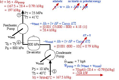
The following revised system diagram corrects both flaws. The steam at the outlet of the HP turbine (port (2)) is reheated to 550°C before entering the LP turbine at port (3). Also the low pressure liquid condensate at port (5) is pumped to a pressure of 800 kPa and passed through a de-aerator prior to being pumped by the feedwater pump to the high pressure of 25 MPa.


This system is referred to as a Reheat cycle, and based on the data above is plotted on the P-h diagram as follows:

Thus we see that in spite of the complexity of the system, the P-h diagram plot enables an intuitive and qualitative initial understanding of the system. Using the methods described earlier in this chapter for analysis of each component, as well as the steam tables, determine the following:
- Assuming that both turbines are adiabatic and neglecting kinetic energy effects determine the combined output power of both turbines [10.6 MW].
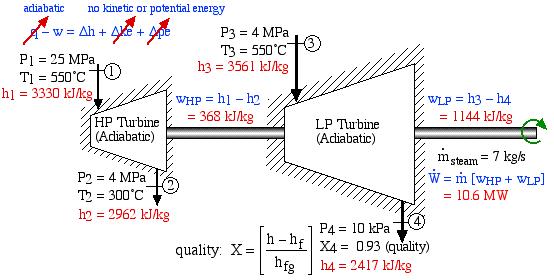
- Assuming that both the condensate pump and the feedwater pump are adiabatic, determine the power required to drive the two pumps [-204 kW].
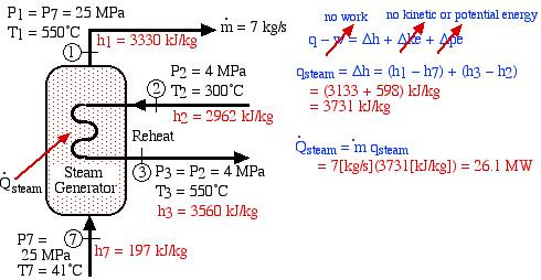
- Determine the total heat transfer to the steam generator, including the reheat system [26.1 MW].
- Determine the overall thermal efficiency of this power plant. (Thermal efficiency (ηth) is defined as the net work done (turbines, pumps) divided by the total heat supplied externally to the steam generator and reheat system) [40 %].
![\eta_{th}=\left[\frac{\dot{W}_{turbines}+\dot{W}_{pumps}}{\dot{Q}_{steam}}\right]=\left[\frac{(10.6-0.2)MW}{26.1MW}\right]=40\%](https://pressbooks.pub/app/uploads/quicklatex/quicklatex.com-7df8e6d4fafb019d5c5d14a7cb8634c4_l3.png "Rendered by QuickLaTeX.com")
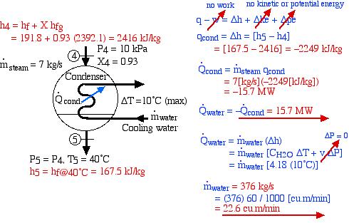
- Determine the heat rejected to the cooling water in the condenser [-15.7 MW].
- Assume that all the heat rejected in the condenser is absorbed by cooling water from the Hocking River. To prevent thermal pollution the cooling water is not allowed to experience a temperature rise above 10°C. If the steam leaves the condenser as saturated liquid at 40°C, determine the required minimum volumetric flow rate of the cooling water [22.6 cubic meters/minute].
- Discuss whether you think that the proposed system can be cooled by the Hocking river. You will need to do some research to determine the minimal seasonal flow in the river in order to validate your decision. (Hint- Google: Hocking River Flow)


(Step 1 above)


![\begin{align*} \color{blue} \dot{W}&\color{blue}=\dot{m}[w_\text{HP} + w_\text{LP}]\\ &\color{red}=10.6 \ \si\MW \end{align*}](https://pressbooks.pub/app/uploads/quicklatex/quicklatex.com-1ed18d1677d2de09027fb46c5d3b03e5_l3.png "Rendered by QuickLaTeX.com")


![\text{quality: } \ X = \left[ \dfrac{h-h_f}{h_{fg}}\right]](https://pressbooks.pub/app/uploads/quicklatex/quicklatex.com-a1cf2910984feaabe7f7354c01b31f73_l3.png "Rendered by QuickLaTeX.com")
(Step 2 above)


![\begin{align*} \color{blue} -w_\text{feed}&\color{blue}=\Delta h=[v \Delta P + C_{H_2O} \Delta T]\\ &\color{red}=[0.001 (25,000-800)+4.18(1)]\\ &\color{red}=28.4 \ \si\kJ/\si\kg\\ \end{align*}](https://pressbooks.pub/app/uploads/quicklatex/quicklatex.com-264e7663e70afd167b8272aecda460e9_l3.png "Rendered by QuickLaTeX.com")
![\begin{align*} \color{blue} -w_\text{cond}&\color{blue}=\Delta h=[v \Delta P + C_{H_2O} \color{red}\cancelto{\color{blue}\Delta T = 0}{\color{blue}\Delta T}\color{blue}]\\ &\color{red}=[0.001(800-10)]=0.79 \ \si\kJ/\si\kg \end{align*}](https://pressbooks.pub/app/uploads/quicklatex/quicklatex.com-9793300ea6c335009c6b57aa3df219c5_l3.png "Rendered by QuickLaTeX.com")

 [\si\kJ/\si\kg]\\ &\color{red}=-204 \ \si\kW\\ \end{align*}](https://pressbooks.pub/app/uploads/quicklatex/quicklatex.com-0a8842c47365a1b94b323910043e9321_l3.png "Rendered by QuickLaTeX.com")
(Step 3 above)


=26.1 \ \si\MW \end{align*}](https://pressbooks.pub/app/uploads/quicklatex/quicklatex.com-f9d8a4a2a24c9d4e01b7c5da4036cbe8_l3.png "Rendered by QuickLaTeX.com")
(Step 6 above)


![\begin{align*} \color{blue} q_\text{cond}&\color{blue}=\Delta h = [h_5-h_4]\\ &\color{red}=[167.5-2416]=-2249 \ \si\kJ/\si\kg \end{align*}](https://pressbooks.pub/app/uploads/quicklatex/quicklatex.com-6b6076dde6db44177328f5735b3f25de_l3.png "Rendered by QuickLaTeX.com")
\\ &\color{red}=-15.7 \ \si\MW \end{align*}](https://pressbooks.pub/app/uploads/quicklatex/quicklatex.com-deeb2ee7dbad8415a1df3e2f98fbe052_l3.png "Rendered by QuickLaTeX.com")

![\begin{align*} \color{blue} \dot{Q}_\text{water}&\color{blue}=\dot{m}_\text{water}(\Delta h)\\ &\color{blue}=\dot{m}_\text{water}[C_{H_2O} \Delta T + v \color{red}\cancelto{\color{blue}\Delta P = 0}{\color{blue}\Delta P}\color{blue}]\\ &\color{blue}=\dot{m}_\text{water}[4.18 (10^\circ\text{C})] \end{align*}](https://pressbooks.pub/app/uploads/quicklatex/quicklatex.com-23d03853d00fa0e305d2f6b9ff34c8df_l3.png "Rendered by QuickLaTeX.com")
![\begin{align*} \color{blue} \dot{m}_\text{water}&\color{red}=376 \ \si\kg/\si\s\\ &\color{blue}=(376) 60/1000 \ [\si{cu\ m}/\si\min]\\ &\color{red}=22.6 \ \si{cu \ m}/\si\min \end{align*}](https://pressbooks.pub/app/uploads/quicklatex/quicklatex.com-37a514404eec95141f828c96178b7f17_l3.png "Rendered by QuickLaTeX.com")
Solved Problem 4.2 – An Open Feedwater Heater added to the Supercritical Steam Power Plant for Athens, Ohio
Thanks to Kris Dambrink from Imtech.nl for making me aware of this alternative approach to adapting an Open Feedwater Heater to a steam power plant (4 Feb 2010).
This Solved Problem is an alternative extension of Solved Proble 4.1 in which we extend the de-aerator by tapping steam from the outlet of the High Pressure turbine and reduce the pressure to 800 kPa by means of a Throttling Control Valve before feeding it into the de-aerator. This allows one to conveniently convert the de-aerator into an Open Feedwater Heater without requiring a bleed tap from the Low Pressure turbine at exactly the de-aerator pressure, as shown in the following diagram:


 : mass fraction


= Feedwater Pump


= Condensate Pump


Note that prior to doing any analysis we always first sketch the complete cycle on a P-h diagram based on the pressure, temperature, and quality data presented on the system diagram. This leads to the following diagram:


On examining the P-h diagram plot we notice the following:
- A mass fraction of the steam y is tapped from the outlet of the HP turbine (2) and passed through the throttle such that its pressure is reduced to that of the de-aerator (9). It is then mixed with a mass fraction (1-y) of the liquid water at station (6). The mass fraction y is chosen to enable the fluid to reach a saturated liquid state at station (7).
- The feedwater pump then pumps the liquid to station (8), thus saving a significant amount of heat from the steam generator in heating the fluid from station (8) to the turbine inlet at station (1). It is true that with a mass fraction of (1-y) there is less power output due to a reduced mass flow rate in the LP turbine, however the net result is normally an increase in thermal efficiency.
Thus once more we see that in spite of the complexity of the system, the P-h diagram plot enables an intuitive and qualitative initial understanding of the system. Using the methods described earlier in this chapter for analysis of each component, as well as the steam tables for evaluating the enthalpy at the various stations (shown in red), and neglecting kinetic and potential energy effects, determine the following:
- Assuming that the open feedwater heater is adiabatic, determine the mass fraction of steam y required to be bled off the outlet of the HP turbine which will bring the fluid from station (6) to a saturated liquid state in the de-aerator. [y = 0.20]We first need to evaluate the enthalpy of the fluid at station (9) after passing through the throttling control valve:


Thus we find that for an ideal throttle the enthalpy h9 = h2 independent of the pressure drop, allowing us to conveniently draw the throttling process as a vertical line on the P-h diagram. We now determine the mass fraction y by considering the mixing process in the open feedwater heater as follows:


Notice that we can estimate this value of y directly from the P-h diagram by simply measuring the enthalpy differences (h7 – h6) and (h9 – h6) with a ruler.
- Assuming that both the condensate pump and the feedwater pump are adiabatic, determine the power required to drive the two pumps [235 kW].On examining the system diagram above we noticed something very strange about the feedwater pump. Until now we considered liquid water to be incompressible, thus pumping it to a higher pressure did not result in an increase of its temperature. However on a recent visit to the Gavin Power Plant we discovered that at 25MPa pressure and more than 100°C water is no longer incompressible, and compression will always result in a temperature increase. We cannot use the simple incompressible liquid formula to determine pump work, however need to evaluate the difference in enthalpy from the Compressed Liquid Water tables, leading to the following results:


![\begin{align*} \color{blue}-w_\text{feed}&\color{blue}=\Delta h = [h_8-h_7]\\ &\color{red}=33 \ \si\kJ/\si\kg \end{align*}](https://pressbooks.pub/app/uploads/quicklatex/quicklatex.com-f3ff4b431ded85adf88ee80ce2b71f3e_l3.png "Rendered by QuickLaTeX.com")


![\begin{align*} \color{blue}-w_\text{cond}&\color{blue}=(1-y) \Delta h\\ &\color{blue}=(1-y)[v \Delta P + C_{H_2O} \color{red}\cancelto{\color{blue}\Delta T = 0}{\color{blue}\Delta T}\color{blue}]\\ &\color{red}=(1-0.20)[0.001(800-10)]\\ &\color{red}=0.63\ \si\kJ/\si\kg \end{align*}](https://pressbooks.pub/app/uploads/quicklatex/quicklatex.com-1806da3635bcc112a0a1c3b5f1921730_l3.png "Rendered by QuickLaTeX.com")
[\si\kJ/\si\kg]\\ &\color{red}=-235\ \si\kW \end{align*}](https://pressbooks.pub/app/uploads/quicklatex/quicklatex.com-12da80da509deda28491913e6f2863d6_l3.png "Rendered by QuickLaTeX.com")
- Assuming that both turbines are adiabatic, determine the new (reduced) combined power output of both turbines. Recall from Solved Problem 4.1 that the power output of the turbines was found to be 10.6 MW if no steam is bled from the LP turbine [8.98 MW]


![\color{teal} \text{quality } \ X_4=\dfrac{\left[h_4-h_{f@10 \ \si\kPa}\right]}{h_{fg@10 \ \si\kPa}}](https://pressbooks.pub/app/uploads/quicklatex/quicklatex.com-3f483040e908d85c0edf4faa1b74d94c_l3.png "Rendered by QuickLaTeX.com")


![\begin{align*} \color{blue} \dot{W}&\color{blue}=\dot{m}\left[w_\text{HP}+w_\text{LP}\right]\\ &\color{red}=8.98 \ \si\MW \end{align*}](https://pressbooks.pub/app/uploads/quicklatex/quicklatex.com-c5507bb93b7f4c993880aa80eb553dba_l3.png "Rendered by QuickLaTeX.com")
Thus as expected we find that the net power output is slightly less than the previous system without the turbine tap. However power control is normally done by changing the feedwater pump speed, and we normally find a liquid water storage tank associated with the de-aerator in order to accommodate the changes in the water mass flow rate. In our case we simply need to increase the water mass flow rate from 7 to 8.25 in order to regain our original power output.
- Determine the total heat transfer to the steam generator, including the reheat system [21.4 MW].


![\begin{align*} \color{blue} \dot{Q}&\color{blue}_\text{steam}=\dot{m} q_\text{steam}\\ &\color{red}=7\left[\si\kg/\si\s\right] (3055\left[\si\kJ/\si\kg\right]) = 21.4\ \si\MW \end{align*}](https://pressbooks.pub/app/uploads/quicklatex/quicklatex.com-14382f320d3874622611312b7feeff74_l3.png "Rendered by QuickLaTeX.com")
- Determine the overall thermal efficiency of this power plant. (Thermal efficiency (ηth) is defined as the net work done (turbines, pumps) divided by the total heat supplied externally to the steam generator and reheat system) [41 %].
![\[\eta_{th}=\left[\frac{\dot{W}_{turbines}+\dot{W}_{pumps}}{\dot{Q}_{steam}}\right]=\left[\frac{(8.98-0.24)MW}{21.4MW}\right]=41\%\]](https://pressbooks.pub/app/uploads/quicklatex/quicklatex.com-05d6fdc022036aec47a58d738a7ff558_l3.png "Rendered by QuickLaTeX.com")
- Determine the heat rejected to the cooling water in the condenser [-12.6 MW].
- Assume that all the heat rejected in the condenser is absorbed by cooling water from the Hocking River. To prevent thermal pollution the cooling water is not allowed to experience a temperature rise above 10°C. If the steam leaves the condenser as saturated liquid at 40°C, determine the required minimum volumetric flow rate of the cooling water [18.1 cubic meters/minute].


![\begin{align*} \color{blue} q&\color{blue}_\text{cond}=\Delta h=[h_5-h_4]\\ &\color{red}=[167.5-2416]=-2249\ \si\kJ/\si\kg \end{align*}](https://pressbooks.pub/app/uploads/quicklatex/quicklatex.com-48a40fddee9b9ba0c2d8534d9171d1ea_l3.png "Rendered by QuickLaTeX.com")
(-2249)[\si\kJ/\si\kg])\\ &\color{red}=-12.6 \ \si\MW \end{align*}](https://pressbooks.pub/app/uploads/quicklatex/quicklatex.com-bc89daf05771bb2d08a422f9d3bae587_l3.png "Rendered by QuickLaTeX.com")

![\begin{align*} \color{blue} \dot{Q}_\text{water}&\color{blue}=\dot{m}_\text{water} (\Delta h)\\ &\color{blue}=\dot{m}_\text{water}\ [C_{H_2O}\Delta T + v\color{red}\cancelto{\color{blue}\Delta P=0}{\color{blue}\Delta P}\color{blue}]\\ &\color{blue}=\dot{m}_\text{water} \ [4.18(10^\circ\text{C})] \end{align*}](https://pressbooks.pub/app/uploads/quicklatex/quicklatex.com-c257f49ce2a7e8420c44e9cbd360ecae_l3.png "Rendered by QuickLaTeX.com")
![\begin{align*} \color{blue} \dot{m}&\color{blue}_\text{water}\color{red}=301 \ \si\kg/\si\s\\ &\color{blue}=(301) 60 / 1000 [\si{cu \ m}/\si\min]\\ &\color{red}=18.1 \ \si{cu \ m}/\si\min \end{align*}](https://pressbooks.pub/app/uploads/quicklatex/quicklatex.com-bea46ea45a40f7e22d2fa24c685d326f_l3.png "Rendered by QuickLaTeX.com")
Note that it is always a good idea to validate ones calculations by evaluating the thermal efficiency using only the heat supplied to the steam generator and that rejected by the condenser.
![\[\eta_{th}=\left[\frac{\dot{Q}_{steam}-\dot{Q}_{cond}}{\dot{Q}_{steam}}\right]=\left[1-\frac{\dot{Q}_{cond}}{\dot{Q}_{steam}}\right]=\left[1-\frac{12.6MW}{21.4MW}\right]=41%\]](https://pressbooks.pub/app/uploads/quicklatex/quicklatex.com-6bed89db0d448e9b0b117554a999db22_l3.png "Rendered by QuickLaTeX.com")
Discussion: Thus we find that the open feedwater heater did in fact raise the efficiency from 40% to 41%. This may not seem like a significant amount, however all the basic components were already in place, since without a de-aerator the steam power plant will deteriorate and become non-functional within a very short time due to leakage of air into the system. Furthermore, if the reduction in power output is not acceptable, then it can be easily remedied by increasing the mass flow rate in the system design. Note that this is a contrived example in order to demonstrate that no matter how complex the system is, we can easily plot the entire system on a P-h diagram and obtain an immediate intuitive understanding and evaluation of the system performance. It is helpful to check each value of enthalpy read or evaluated from the steam tables and compare them to the values on the enthalpy axis of the P-h diagram.
Refrigerators and Heat Pumps
Introduction and Discussion
In the early days of refrigeration the two refrigerants in common use were ammonia and carbon dioxide. Both were problematic – ammonia is toxic and carbon dioxide requires extremely high pressures (from around 30 to 200 atmospheres!) to operate in a refrigeration cycle, and since it operates on a transcritical cycle the compressor outlet temperature is extremely high (around 160°C). When Freon 12 (dichloro-diflouro-methane) was discovered it totally took over as the refrigerant of choice. It is an extremely stable, non toxic fluid, which does not interact with the compressor lubricant, and operates at pressures always somewhat higher than atmospheric, so that if any leakage occurred, air would not leak into the system, thus one could recharge without having to apply vacuum.
Unfortunately when the refrigerant does ultimately leak and make its way up to the ozone layer the ultraviolet radiation breaks up the molecule releasing the highly active chlorine radicals, which help to deplete the ozone layer. Freon 12 has since been banned from usage on a global scale, and has been essentially replaced by chlorine free R134a (tetraflouro-ethane) – not as stable as Freon 12, however it does not have ozone depletion characteristics.
Recently, however, the international scientific consensus is that Global Warming is caused by human energy related activity, and various man made substances are defined on the basis of a Global Warming Potential (GWP) with reference to carbon dioxide (GWP=1). R134a has been found to have a GWP of 1300 and in Europe, within a few years, automobile air conditioning systems will be barred from using R134a as a refrigerant.
The new hot topic is a return to carbon dioxide (R744) as a refrigerant (refer for example to the website: R744.com). The previous two major problems of high pressure and high compressor temperature are found in fact to be advantageous. The very high cycle pressure results in a high fluid density throughout the cycle, allowing miniaturization of the systems for the same heat pumping power requirements. Furthermore the high outlet temperature will allow instant defrosting of automobile windshields (we don’t have to wait until the car engine warms up) and can be used for combined space heating and hot water heating in home usage (refer for example: Norwegian IEA Heatpump Program Annex28.
A Basic R134a Vapor-Compression Refrigeration System
Unlike the situation with steam power plants it is common practice to begin the design and analysis of refrigeration and heat pump systems by first plotting the cycle on the P-h diagram.
The following schematic shows a basic refrigeration or heat pump system with typical property values. Since no mass flow rate of the refrigerant has been provided, the entire analysis is done in terms of specific energy values. Notice that the same system can be used either for a refrigerator or air conditioner, in which the heat absorbed in the evaporator (qevap) is the desired output, or for a heat pump, in which the heat rejected in the condenser (qcond) is the desired output.


In this example we wish to evaluate the following:
- Heat absorbed by the evaporator (qevap)
![\left[\frac{kJ}{kg}\right]](https://pressbooks.pub/app/uploads/quicklatex/quicklatex.com-f50733e1f4cc71bb4487402b1b67771f_l3.png "Rendered by QuickLaTeX.com")
- Heat rejected by the condenser (qcond)
- Work done to drive the compressor (wcomp)
- Coefficient of Performance (COP) of the system, either as a refrigerator or as a heat pump.
As with the Steam Power Plant, we find that we can solve each component of this system separately and independently of all the other components, always using the same approach and the same basic equations. We first use the information given in the above schematic to plot the four processes (1)-(2)-(3)-(4)-(1) on the P-h diagram. Notice that the fluid entering and exiting the condenser (State (2) to State (3)) is at the high pressure 1 MPa. The fluid enters the evaporator at State (4) as a saturated mixture at -20°C and exits the evaporator at State (1) as a saturated vapor. State (2) is given by the intersection of 1 MPa and 70°C in the superheated region. State (3) is seen to be in the subcooled liquid region at 30°C, since the saturation temperature at 1 MPa is about 40°C. The process (3)-(4) is a vertical line (h3 = h4) as is discussed below.
In the following section we develop the methods of evaluating the solution of this example using the R134a refrigerant tables. Notice that the refrigerant tables do not include the subcooled region, however since the constant temperature line in this region is essentially vertical, we use the saturated liquid value of enthalpy at that temperature.


Notice from the P-h diagram plot how we can get an instant visual appreciation of the system performance, in particular the Coefficient of Performance of the system by comparing the enthalpy difference of the compressor (1)-(2) to that of the evaporator (4)-(1) in the case of a refrigerator, or to that of the condenser (2)-(3) in the case of a heat pump.
We now consider each component as a separate control volume and apply the energy equation, starting with the compressor. Notice that we have assumed that the kinetic and potential energy change of the fluid is negligible, and that the compressor is adiabatic. The required values of enthalpy for the inlet and outlet ports are determined from the R134a refrigerant tables.


![\begin{align*} \color{red}\cancelto{\color{blue}\text{adiabatic}}{\color{blue}q}\color{blue}-w&\color{blue}= \Delta h + \Delta \color{red}\cancelto{\color{blue}\text{no kinetic or potential energy}}{\color{blue} ke}\color{blue}+\Delta \color{red}\cancelto{}{\color{blue}pe}\\ \color{blue} -w&\color{blue}=\Delta h\\ &\color{blue}=h_2-h_1\color{red}=[303.9-238.4]\ \si\kJ/\si\kg\\ \color{red}-w_\text{comp}&\color{red}=65.5\ \si\kJ/\si\kg \end{align*}](https://pressbooks.pub/app/uploads/quicklatex/quicklatex.com-fbe0f5c451e8225af720923b00b2ce32_l3.png "Rendered by QuickLaTeX.com")
The high pressure superheated refrigerant at port (2) is now directed to a condenser in which heat is extracted from the refrigerant, allowing it to reach the subcooled liquid region at port (3). This is shown on the following diagram of the condenser:

![\begin{align*} \color{red}\cancelto{\color{blue}\text{adiabatic}}{\color{blue}q}\color{blue}-w&\color{blue}= \Delta h + \Delta \color{red}\cancelto{\color{blue}\text{no kinetic or potential energy}}{\color{blue} ke}\color{blue}+\Delta \color{red}\cancelto{}{\color{blue}pe}\\ \color{blue} q&\color{blue}=\Delta h = [h_3-h_2]\\ &\color{red}=[93.6-303.9]\ \si\kJ/\si\kg \end{align*}](https://pressbooks.pub/app/uploads/quicklatex/quicklatex.com-d6fabee3ad4cb7b0323bf31dad9bd63d_l3.png "Rendered by QuickLaTeX.com")


The throttle is simply an expansion valve which is adiabatic and does no work, however enables a significant reduction in temperature of the refrigerant as shown in the following diagram:


The final component is the evaporator, which extracts heat from the surroundings at the low temperature allowing the refrigerant liquid and vapor mixture to reach the saturated vapor state at station (1).

![\begin{align*} \color{blue} q&\color{red}\cancelto{\color{blue}\text{no work}}{\color{blue}-w} \color{blue} = \Delta h + \Delta \color{red}\cancelto{\color{blue}\text{no kinetic or potential energy}}{\color{blue} ke}\color{blue}+\Delta \color{red}\cancelto{}{\color{blue}pe}\\ \color{blue}q&=\color{blue}\Delta h = [h_1-h_4]\\ &\color{red}=[238.4-93.6] \ \si\kJ/\si\kg \end{align*}](https://pressbooks.pub/app/uploads/quicklatex/quicklatex.com-052b8c7c5380250211a1ea1111466f59_l3.png "Rendered by QuickLaTeX.com")


In determining the Coefficient of Performance – for a refrigerator or air-conditioner the desired output is the evaporator heat absorbed, and for a heat pump the desired output is the heat rejected by the condenser which is used to heat the home. The required input in both cases is the work done on the compressor (i.e. the electricity bill). Thus


Notice that for the same system we always find that COPHP = COPR + 1.
Notice also that the COP values are usually greater than 1, which is the reason why they are never referred to as “Efficiency” values, which always have a maximum of 100%.
Thus the P-h diagram is a widely used and very useful tool for doing an approximate evaluation of a refrigerator or heat pump system. In fact, in the official Reference Handbook supplied by the NCEES to be used in the Fundamentals of Engineering exam, only the P-h diagram is presented for R134a. You are expected to answer all the questions on this subject based on plotting the cycle on this diagram as shown above.
Solved Problem 4.3 – A Home Geothermal Heat-Pump
Introduction and Description
With the global quest for energy efficiency, there is renewed interest in Geothermal Heat Pumps which were have been in limited use for more than 60 years. Essentially this technology relies on the fact that a few meters below the surface of the earth the temperature remains relatively constant throughout the year (around 55°F (13°C)), warmer than the air above it during winter, and cooler during summer. This means that we can design a heat pump which can combine hot water and space heating in winter in which the earth is used as a heat source (rather than the outside air) at a considerable increase in coefficient of performance COP. Similarly, with suitable valving, we can use the same system in summer for hot water heating and air conditioning in which the earth is used as a heat sink, rather than the outside air. This is achieved by using a Ground Loop in order to enable heat transfer with the earth, as described in the USDOE website: Geothermal Heat Pumps. Another description of geothermal heat pumps has been provided by David White Services of Southeastern Ohio and includes a YouTube video by WaterFurnace: GEOTHERMAL How does it work.
Problem
We wish to do a preliminary thermodynamic analysis of the following home geothermal heat pump system designed for wintertime hot water and space heating. Notice that with suitable valving this system can be used both in winter for space heating and in summer for air conditioning, with hot water heating throughout the year.


Notice that the condenser section includes both the hot water and space heater and station (3) is specified as being in the Quality region. Assume that 50°C is a reasonable maximum hot water temperature for home usage, thus at a high pressure of 1.6 MPa, the maximum power available for hot water heating will occur when the refrigerant at station (3) reaches the saturated liquid state. (Quick Quiz: justify this statement). Assume also that the refrigerant at station (4) reaches a subcooled liquid temperature of 20°C while heating the air.
- Using the R134a property tables determine the enthalpies at all five stations and verify and indicate their values on the P-h diagram.
- Station 1 we get from the saturated vapor pressure table: hg = 253.8

- Station 2 we get from the superheated vapor table : h = 293.3
- Station 3 we get from the saturated liquid pressure table: hf = 136
- Station 4 we approximate as a saturated liquid at 20°C: h= 79.32
- Station 5 is the same as station 4 since the only part in between is an adiabatic throttle: h= 79.32
- Station 1 we get from the saturated vapor pressure table: hg = 253.8
- Determine the mass flow rate of the refrigerant R134a.
- The mass flow rate is determined by the compressor which puts 500W of power into the system. We can find the mass flow rate by using the power from the pump and dividing it by the difference in enthalpy across the compressor (between Stations 1 & 2):
![\[\dot{m}=\frac{-0.5\frac{kJ}{s}}{253.8\frac{kJ}{kg}-293.3\frac{kJ}{kg}}=\frac{-0.5\frac{kJ}{s}}{-39.5\frac{kJ}{kg}}=0.0127\frac{kg}{s}\]](https://pressbooks.pub/app/uploads/quicklatex/quicklatex.com-ad8febb0b8deffb6b669de2461e99d49_l3.png "Rendered by QuickLaTeX.com")
- The mass flow rate is determined by the compressor which puts 500W of power into the system. We can find the mass flow rate by using the power from the pump and dividing it by the difference in enthalpy across the compressor (between Stations 1 & 2):
- Determine the power absorbed by the hot water heater and that absorbed by the space heater.
- At this point we know the mass flow rate and the enthalpies at each station so finding the power absorbed by the water heater and space heater is as simple as finding the difference in enthalpies across each component and multiplying by the mass flow rate:
![\[P_{WH}=0.0127\frac{kg}{s}*(293.3\frac{kJ}{kg}-136\frac{kJ}{kg})=2.0kW\]](https://pressbooks.pub/app/uploads/quicklatex/quicklatex.com-8994eff0dfb6f54d218fd416a7411dfb_l3.png "Rendered by QuickLaTeX.com")
![\[P_{SH}=0.0127\frac{kg}{s}*(136\frac{kJ}{kg}-79.32\frac{kJ}{kg})=720W\]](https://pressbooks.pub/app/uploads/quicklatex/quicklatex.com-266923da5326297b072ce79f64a541aa_l3.png "Rendered by QuickLaTeX.com")
- At this point we know the mass flow rate and the enthalpies at each station so finding the power absorbed by the water heater and space heater is as simple as finding the difference in enthalpies across each component and multiplying by the mass flow rate:
- Determine the time taken for 100 liters of water at an initial temperature of 20°C to reach the required hot water temperature of 50°C.
- We know one liter of water has a mass of 1kg so total mass of the 100 L is 100 kg and from the steam tables we can approximate the change in enthalpy of water over this 30 degree change in temperature to be 125.4 so we can use these numbers along with our power from the previous step:
![\[\frac{100kg*125.4\frac{kJ}{kg}}{2kW}=6270s\,\text{or}\,104.5min\]](https://pressbooks.pub/app/uploads/quicklatex/quicklatex.com-3256ac622d046a96e11857f1a9b784bc_l3.png "Rendered by QuickLaTeX.com")
- We know one liter of water has a mass of 1kg so total mass of the 100 L is 100 kg and from the steam tables we can approximate the change in enthalpy of water over this 30 degree change in temperature to be 125.4
- Determine the Coefficient of Performance of the hot water heater (defined as the heat absorbed by the hot water divided by the work done on the compressor)
![\[COP=\frac{Q}{W}\]](https://pressbooks.pub/app/uploads/quicklatex/quicklatex.com-c1c07d5f409fc72dbc43e4171b0a6d19_l3.png "Rendered by QuickLaTeX.com")
![\[COP_{HW}=\frac{2kW}{0.5kW}=4.0\]](https://pressbooks.pub/app/uploads/quicklatex/quicklatex.com-81b8a8e53e0eb8dd1349dd7a4364ec56_l3.png "Rendered by QuickLaTeX.com")
- Determine the Coefficient of Performance of the heat pump (defined as the total heat rejected by the refrigerant in the hot water and space heaters divided by the work done on the compressor)
![\[COP_{HP}=\frac{2kW+0.72kW}{0.5kW}=5.44\]](https://pressbooks.pub/app/uploads/quicklatex/quicklatex.com-34ceb011290fc893fb374c94732c468a_l3.png "Rendered by QuickLaTeX.com")
- Think about what changes would be required of the system parameters if no geothermal water loop was used, and the evaporator was required to absorb its heat from the outside air at -10°C. Discuss the advantages of the geothermal heat pump system over other means of space and water heating.
