20
Defining and Evaluating Entropy
Defining Entropy (S) through the Clausius Inequality
Consider two heat engines, one a reversible (Carnot) engine and the other an irreversible heat engine. For purposes of developing the Clausius Inequality we assume that both engines are sized to accept the same amount of heat QH from the thermal source. Thus since the irreversible engine must be less efficient than the Carnot engine, it must reject more heat QL,irrev to the thermal sink than that rejected by the Carnot engine QL,rev, as shown:

 (heat source)


 (heat sink)


Consider first the reversible (Carnot) heat Engine. We saw in Chapter 5 that reversible heat transfer can only occur isothermally, thus the cyclic integral of the heat transfer divided by the temperature can be evaluated as follows:
![\[\oint\frac{\delta Q}{T} = \frac{Q_H}{T_H}-\frac{Q_{L,rev}}{T_L}\]](https://pressbooks.pub/app/uploads/quicklatex/quicklatex.com-20b01352c13979a1e984530d52b181c8_l3.png "Rendered by QuickLaTeX.com")
Recall from Chapter 5 that whenever we considered the efficiency of a reversible heat engine, we went into “meditation mode”, replacing the ratio of heat flows with the ratio of temperatures:

![\xRightarrow[\dfrac{Q_\text{L}}{Q_\text{H}}=\dfrac{T_\text{L}}{T_\text{H}}]{+ \ +} \dfrac{Q_\text{L,rev}}{T_\text{L}}=\dfrac{Q_\text{H}}{T_\text{H}}, \ \text{thus: } \color{red}\boxed{\color{black}\displaystyle \oint\dfrac{\delta Q}{T} =0}](https://pressbooks.pub/app/uploads/quicklatex/quicklatex.com-2c12843be0504bc3902b212c285f6939_l3.png "Rendered by QuickLaTeX.com")
Notice from the above diagram showing the two heat engines that for an irreversible engine having the same value of heat transfer from the thermal source QH as the reversible engine, the heat transfer to the thermal sink QL,irrev> QL,rev.
Let Qdiff = (QL,irrev – QL,rev), then the cyclic integral for an irreversible heat engine becomes:
![\[\oint\frac{\delta Q}{T}=\frac{Q_H}{T_H} - \left(\frac{Q_{L,rev}}{T_L}+\frac{Q_{\diff}}{T_L}\right) < 0\]](https://pressbooks.pub/app/uploads/quicklatex/quicklatex.com-1e233b88b32f63190269a28dbb894873_l3.png "Rendered by QuickLaTeX.com")
Thus finally, for any reversible or irreversible heat engine we obtain the Clausius Inequality:
![\[\oint\frac{\delta Q}{T}\leq0\]](https://pressbooks.pub/app/uploads/quicklatex/quicklatex.com-5bfa52c4bf5ec35efef7ba635a4eb64b_l3.png "Rendered by QuickLaTeX.com")
Defining the Property Entropy – S
All properties (such as pressure P, volume V, etc.) have a cyclic integral equal to zero.


A very strange definition indeed, and difficult to comprehend. It is defined in differential format as the reversible heat transfer divided by the temperature. In an attempt to try and understand it we rewrite the definition as follows:
Heat: 
It is advantageous to compare this definition with the equivalent definition of work as follows:
Work: 
Thus it begins to make sense. Work done requires both a driving force (pressure P) and movement (volume change dV). We implicitly evaluated the work done for reversible processes – always neglecting friction or any other irreversibility. Similarly we can state that heat transfer requires both a driving force (temperature T) and some equivalent form of “movement” (entropy change dS). Since temperature can be considered as represented by the vibration of the molecules, it is this transfer of vibrational energy that we define as entropy.
Increase in Entropy Principle 
We now continue with the Increase in Entropy Principle which is also derived from the Clausius Inequality, and states that for any process, the total change in entropy of a system or control volume together with its enclosing adiabatic surroundings is always greater than or equal to zero. This total change of entropy is denoted the Entropy Generated during the process (Sgen ![\left[\frac{kJ}{K}\right]](https://pressbooks.pub/app/uploads/quicklatex/quicklatex.com-fe6842fc4377b1c086e55b40ce0cd042_l3.png "Rendered by QuickLaTeX.com") or sgen
or sgen ![\left[\frac{kJ}{kg\times K}\right])](https://pressbooks.pub/app/uploads/quicklatex/quicklatex.com-8c67925bc249a3bea582cec7bd6e0e70_l3.png "Rendered by QuickLaTeX.com") . For reversible processes the entropy generated will always be zero.
. For reversible processes the entropy generated will always be zero.
1. Non-flow Process
We previously found from considerations of the Clausius Inequality that the following cyclic integral is always less than or equal to zero, where the equality occurred for a reversible cycle.
This lead to the definition of the property Entropy (S). Consider now an irreversible cycle in which process (1) -> (2) follows an irreversible path, and process (2) -> (1) a reversible path, as shown:
Thus the entropy change of an adiabatic process is always greater than or equal to zero, where the equality applies to reversible processes. However not all processes are adiabatic. Nevertheless we can always enclose a system in a surrounding environment which is adiabatic, thus considering the total entropy change of both the system and surroundings we obtain:


Thus the Increase in Entropy Principle states that for any process the total change in entropy of a system together with its enclosing adiabatic surroundings is always greater than or equal to zero. This total change of entropy is denoted the Entropy Generated during the process (Sgen or sgen .
2. Flow Processes (Steady Flow)
We now consider the entropy generated during a steady flow process through a single-input/single-output Control Volume (CV) enclosed in an adiabatic surroundings as shown:


Notice that for a steady flow system there can be no change of any of its property values with time, thus the rate of increase of entropy can only be associated with the surroundings. Notice also that at station (2) we are also dumping entropy from the control volume into the surroundings, and at station (1) we are sucking entropy out of the surroundings, leading to:


Surprisingly the form of the specific entropy generated function sgen for a control volume is identical to that for a system.
For multiple-input, multiple-output control volumes under steady flow conditions, the entropy generated function is extended to:
![\[\dot{S}_{gen}= \sum_e \dot{m}_es_e-\sum_i\dot{m}_is_i+\frac{\dot{Q}_{surr}}{T_0}\geq 0\,\,\,\,\,\,\,\left(\dot{Q}_{surr}=-\dot{Q}\right)\]](https://pressbooks.pub/app/uploads/quicklatex/quicklatex.com-4eabb0cb32fe425720bfd1e84ec285ce_l3.png "Rendered by QuickLaTeX.com")
where the summations ( ) are taken over all the exit ports (e) and inlet ports (i).
Evaluating Entropy (The T ds relations)
We use the differential form of the energy equation to derive the Tds relations which can be used to evaluate the change of entropy (Δs) for processes involving 2-phase fluids (Steam, R134a, CO2), solids or liquids, or ideal gasses.
That is “Tedious”, but without the vowels, of course! Recall from consideration of the Clausius Inequality that we defined entropy as follows:
Define Entropy:  thus:
thus: 
Consider the differential form of the system energy equation:

Also, from the definition of enthalpy h:

Tables of 2-phase fluid (Steam, R134a)

Notice that all the properties on the right hand side of this equation T, P, v, u are measurable properties given in the tables, thus this differential equation can be solved numerically, leading to the table values of entropy s.
Liquid (or solid-incompressible)


Ideal Gas


Finally we present a convenient Entropy Equation Summary Sheet which summarizes the relevant relations concerning entropy generation and evaluation of entropy change Δs. The Isentropic Processes Summary Sheet extends the relations of entropy change to enable the evaluation of isentropic processes.
One of the important applications of isentropic processes is in determining the efficiency of various adiabatic components. These include turbines, compressors and aircraft jet nozzles. Thus we have made the statement that steam turbines are designed to be adiabatic, and that any heat loss from the turbine will result in a reduction in output power, however only now can we make the statement that the ideal turbine is isentropic. This enables us to evaluate the Adiabatic Efficiency (sometimes referred to as isentropic efficiency) of these components, and we extend the isentropic process sheet with an Adiabatic Efficiency Summary Sheet.
There are two property diagrams involving entropy in common usage, the temperature-entropy (T-s) and enthalpy-entropy (h-s) “Mollier” diagrams. We will find that the h-s diagram is extremely useful for evaluating adiabatic turbines and compressors, and complements the P-h diagram which we used in Chapter 4 to evaluate entire steam power plants or refrigerator systems. The h-s diagram for steam is presented below:


![\text{Enthalpy}\left[\si\kJ/\si\kg\right]](https://pressbooks.pub/app/uploads/quicklatex/quicklatex.com-5f9ba42a2589ecf8927c1022e94d51cb_l3.png "Rendered by QuickLaTeX.com")
![\text{Entropy}\left[\si\kJ/\si{kg\ K}\right]](https://pressbooks.pub/app/uploads/quicklatex/quicklatex.com-fc79eecebd59edad421c610253bf5c20_l3.png "Rendered by QuickLaTeX.com")
![\text{Pressure} \left[\si\MPa\right]](https://pressbooks.pub/app/uploads/quicklatex/quicklatex.com-9359ba3e10c9dd21e37d6e5216a220aa_l3.png "Rendered by QuickLaTeX.com")


![\text{Quality}\left[\%\right]](https://pressbooks.pub/app/uploads/quicklatex/quicklatex.com-9e2b8c826fa58083002b97c4dc856bd0_l3.png "Rendered by QuickLaTeX.com")
The important characteristic of the h-s diagram is that the ideal adiabatic turbine can be conveniently plotted as a vertical line, allowing an intuitive visual appreciation of the turbine performance. We define the turbine adiabatic efficiency as follows:


Notice that for the actual turbine there will always be an increase in entropy, which means that the turbine adiabatic efficiency will always be less than 100%.
An Adiabatic Steam Turbine Example
Consider an adiabatic steam turbine having a turbine adiabatic efficiency ηT = 80%, operating under the conditions shown in the following diagram:


- Using steam tables, determine the enthalpy and entropy values at station (1) and station (2s) assuming that the turbine is isentropic. [h1 = 3479
 , s1 = 7.764
  ; h2s = 2461 , s2s = s1]
 - From the definition of turbine adiabatic efficiency (shown on the diagram), and given that ηT = 80%, determine the actual enthalpy and entropy values as well as the temperature at station (2a). [h2a = 2665 kJ/kg, s2a = 8.38 kJ/kg.K, T2a = 88°C]
- Plot the actual and isentropic turbine processes (Stations (1)-(2a) and (1)-(2s)) on the enthalpy-entropy h-s “Mollier” diagram, and indicate the actual turbine specific work (wa) as well as the isentropic turbine specific work (ws) on the diagram.
- Determine the actual power output of the turbine (kW). [1629 kW]
The h-s diagram plot follows. Notice that we have indicated all the enthalpy and entropy values (which we determined from the steam tables) on the plot. This allows a check on the feasibility of our results.


Aircraft Gas Turbine Engines
There are many different forms and modifications of aircraft gas turbine engines, and in this course we discuss two variants – the ideal turbojet engine, and the gas turbine engine for usage in helicopters.

The ideal turbojet engine shown schematically in the above figure comprises the series connection of five components – diffuser, compressor, combustor, turbine, and nozzle. The analysis of the complete system, is best done in terms of the h-s (enthalpy-entropy) diagram, which we will develop in class. Throughout the system we assume that the fluid is pure air, and the combustors are considered to be constant-pressure heat-addition devices. Notice that the sole purpose of the turbine is to drive the compressor, the nozzle providing the final kinetic energy increase to drive the aircraft.
The gas turbine engine for usage in helicopters is shown below:

In this case we see that there is no diffuser or nozzle, and that the turbine section has been replaced by two independent turbines – a “gas generator”, or “gassifier” turbine to drive the compressor, and an output turbine to drive the helicopter blades. A typical gas turbine engine of this type is the General Electric T700 engine shown below, which is used in the Army Black Hawk helicopter.


Solved Problem – A Supercritical Steam Power Plant for Athens, Ohio
Consider a supercritical steam power plant with reheat for Athens, Ohio:


In this exercise we wish to evaluate the high pressure (HP) and low pressure (LP) turbines of this system (circled in red), both of which are assumed to be adiabatic.
- Plot the two turbine processes (Stations (1)-(2) and (3)-(4)) on the enthalpy-entropy h-s “Mollier” diagram. Plot also the equivalent isentropic turbine processes on the diagram, and indicate the actual turbine specific work as well as the isentropic turbine specific work for both turbines on the h-s diagram.
- Using steam tables, determine the turbine adiabatic efficiency ηT of both turbines.
- Discuss your results as well as the feasibility of the turbine set.
Justify all values used and derive all equations used starting from the basic energy equation for a flow system, the basic definition of turbine adiabatic efficiency ηT.
Solution Approach:
- Plot the two turbine processes (Stations (1)-(2) and (3)-(4)) on the enthalpy-entropy h-s “Mollier” diagram. Plot also the equivalent isentropic turbine processes on the diagram, and indicate the actual turbine specific work as well as the isentropic turbine specific work for both turbines on the h-s diagram. [refer h-s diagram below]
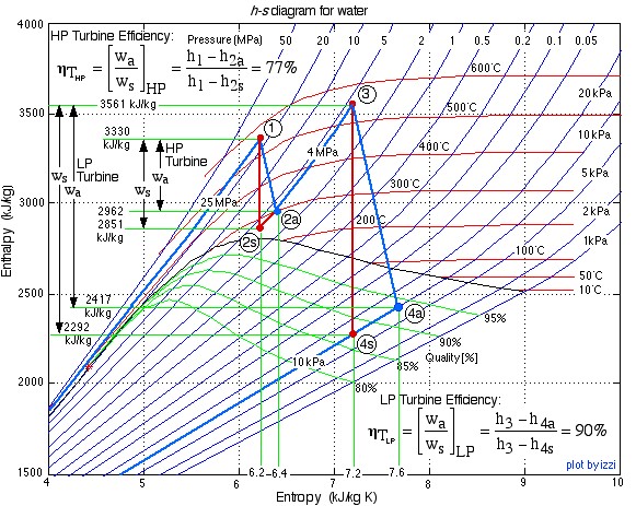
![\eta_{T _\text{HP}}= \left[\dfrac{w_\text{a}}{w_\text{s}}\right]_\text{HP} = \dfrac{h_1-h_\text{2a}}{h_1-h_\text{2s}}=77\%](https://pressbooks.pub/app/uploads/quicklatex/quicklatex.com-575d7ffeadfa170896507a430340ee67_l3.png "Rendered by QuickLaTeX.com")


![\eta_{T _\text{LP}}= \left[\dfrac{w_\text{a}}{w_\text{s}}\right]_\text{LP} = \dfrac{h_3-h_\text{4a}}{h_3-h_\text{4s}}=90\%](https://pressbooks.pub/app/uploads/quicklatex/quicklatex.com-16a627fad8950aab8fda7adf20dda9e5_l3.png "Rendered by QuickLaTeX.com")
- Using steam tables, determine the turbine adiabatic efficiency ηT of both turbines.
- Discuss your results as well as the feasibility of the turbine set.

